What Is a Bonding Curve in Crypto?

Key Takeaways

Bonding curves represent a fundamental mathematical framework in the cryptocurrency industry, establishing a direct relationship between token supply and price through automated mechanisms. By creating a predictable correlation between these two variables, bonding curves enable projects to manage token distribution, pricing, and liquidity in a transparent and algorithmic manner.

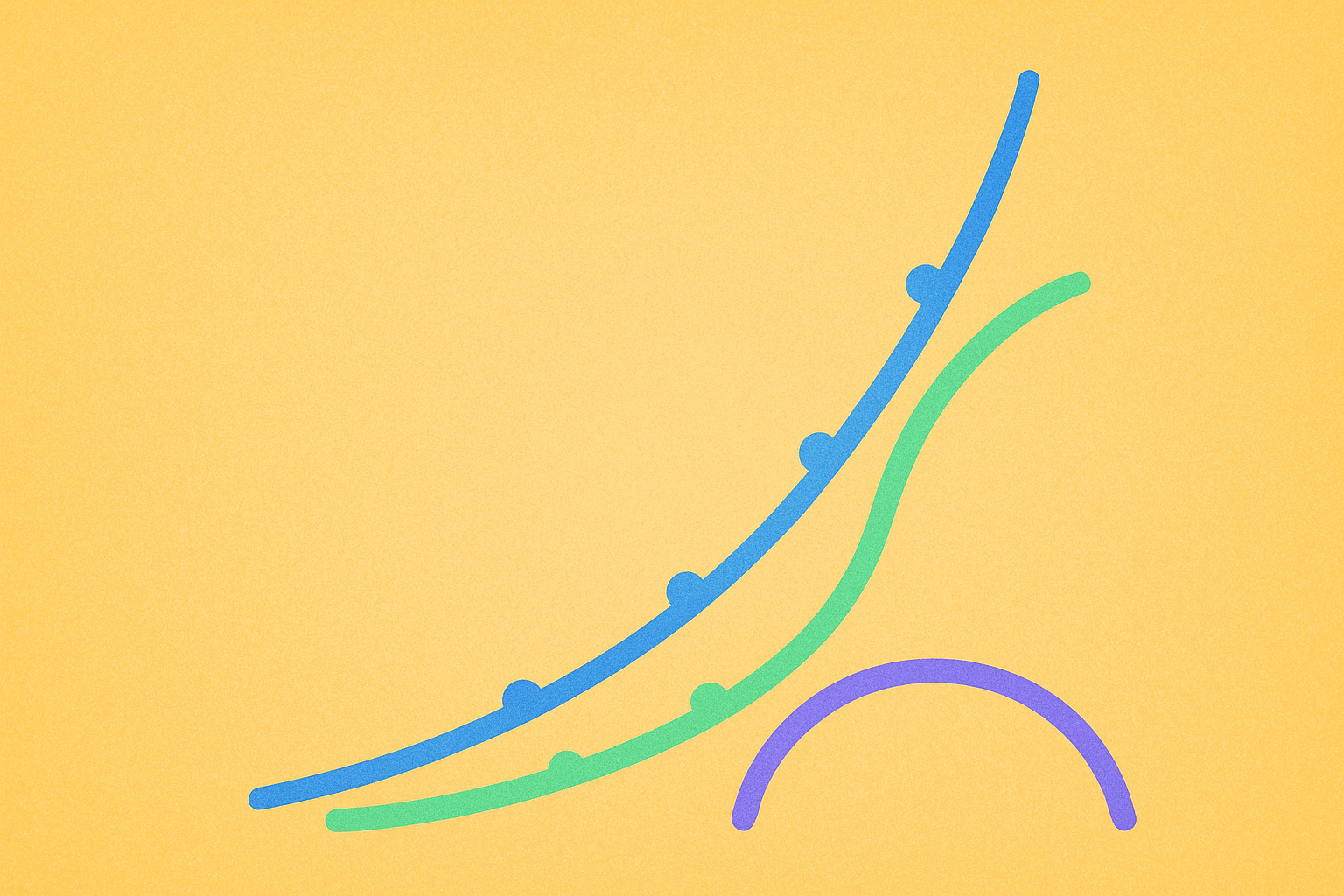
Projects have the flexibility to customize their token economics by implementing different curve types, each serving distinct strategic purposes. Linear curves offer steady, predictable growth; exponential curves reward early adopters with potentially higher returns; logarithmic curves provide initial rapid growth that stabilizes over time; and specialized curves like step-functions or S-curves can address specific project needs.

While bonding curves provide structure and automation to token markets, they do not guarantee complete self-sustainability. Token volatility, market sentiment, and external factors can influence outcomes beyond the mathematical model. However, platforms like pump.fun demonstrate the practical viability of bonding curves, showing how they can facilitate predictable token issuance, enable early market participation, and create functional decentralized markets driven by supply and demand dynamics.

Introduction

Supply and demand have served as foundational economic principles for centuries, influencing markets across diverse asset classes. From precious metals and rare collectibles to everyday commodities, these principles determine value and drive pricing mechanisms. The question arises: how can these time-tested concepts be effectively applied to the cryptocurrency industry, where assets exist entirely in digital form without physical scarcity?

The cryptocurrency landscape is built upon numerous mathematical concepts and algorithmic frameworks. Among these, bonding curves stand out as a particularly significant mechanism that defines the relationship between the price and supply of digital assets. This mathematical model creates a systematic approach to token valuation and distribution.

In a traditional bonding curve implementation, token prices tend to increase as more tokens are purchased and enter circulation. Conversely, when tokens are sold or removed from circulation, prices typically decrease. This dynamic creates a mechanism that often benefits early market participants and active traders who can capitalize on price movements.

Bonding curves have become an essential component of tokenomics, the economic model governing cryptocurrency projects. Their importance is evident in the success of platforms like pump.fun, which leverages bonding curve mechanisms to automate pricing strategies, manage liquidity pools, and control token distribution processes.

Given the growing significance of bonding curves in decentralized finance and token launches, this article explores their fundamental function, examines different types of curves and their characteristics, and analyzes their broader importance in shaping the cryptocurrency industry.

What Are Bonding Curves?

Bonding curves are mathematical models designed to establish a direct and predictable correlation between the supply of cryptocurrency assets and their market price. These models operate through algorithmic governance, meaning that a predefined mathematical formula automatically adjusts an asset's price based on changes in its circulating supply.

This concept mirrors how resources have been valued throughout economic history. When demand for a scarce resource increases while its availability remains limited or fixed, market forces typically drive the price upward. Bonding curves apply this same fundamental principle to digital asset markets, creating an automated system that adjusts token prices in response to supply changes.

The implementation of bonding curves relies on smart contracts, which are self-executing programs deployed on blockchain networks. These smart contracts manage the pricing mechanism, ensuring that bonding curve operations are automatic, transparent, and decentralized. This removes the need for centralized intermediaries or manual price adjustments, creating a trustless system where price changes follow predetermined mathematical rules.

The transparency of blockchain technology means that anyone can verify the bonding curve formula and predict how prices will change as supply fluctuates. This predictability is a key advantage, as it allows market participants to make informed decisions based on mathematical certainty rather than speculation about arbitrary price changes.

How Do Bonding Curves Work?

The fundamental operating principle behind bonding curves is straightforward yet powerful: as more tokens are purchased, the circulating supply increases, which typically results in a price increase according to the curve's formula. Conversely, when tokens are sold back to the bonding curve, the circulating supply decreases, causing the price to decline proportionally.

To illustrate this mechanism in practice, consider a hypothetical scenario where a new project launches tokens using a bonding curve system. In the initial phase, when the circulating supply is minimal, early adopters who purchase tokens will likely acquire them at relatively low prices. This creates an incentive for early participation and risk-taking.

As the project gains traction and attracts more attention, additional traders begin purchasing tokens. This increased demand causes the circulating supply to grow, and the bonding curve may mint new tokens according to its programmed formula. As supply expands, the bonding curve automatically increases the price, reflecting the growing market interest and token scarcity relative to demand.

The automated nature of bonding curves provides continuous liquidity, as the smart contract is always available to facilitate token purchases and sales. Unlike traditional markets where liquidity depends on finding counterparties willing to trade, bonding curves act as an algorithmic market maker, always ready to transact at the current curve-determined price.

Projects can customize their bonding curve tokenomics by selecting and implementing different mathematical models that define unique curve shapes and behaviors. There is theoretically no limit to the types of curves that can be designed, but several common patterns have emerged in practice, including linear, exponential, and logarithmic curves, each with distinct characteristics and use cases.

Linear Bonding Curves

The linear bonding curve represents the most straightforward mathematical model for implementing this mechanism. In a linear curve system, the price of a token increases in direct, proportional relationship to the number of tokens sold and the total supply of tokens in circulation.

Under this model, the price increment is fixed and predetermined. For every new token minted or sold through the bonding curve, the price increases by the same constant amount. For example, if the price increase is set at 0.01 units per token, the first token might cost 1.00, the second 1.01, the third 1.02, and so on, creating a steady, predictable price progression.

Linear bonding curves are particularly useful for projects seeking predictability and simplicity in their token economics. They create a transparent pricing structure where participants can easily calculate future prices based on supply projections. This transparency can build trust and reduce speculation about arbitrary price changes.

Exponential Bonding Curves

Exponential bonding curves create a more aggressive pricing model where the token price depends exponentially on the circulating supply. This means that price increases accelerate as more tokens are purchased, rather than growing at a constant rate.

In an exponential curve system, if tokens are purchased at double the previous rate, the price will more than double, potentially becoming significantly more expensive much faster than in a linear model. This creates a steep price curve that rewards early participants disproportionately.

Exponential curves are typically employed by projects that want to strongly incentivize early participation and risk-taking. Early buyers who enter when prices are low may face significant uncertainty about the project's success, but they also stand to profit substantially if the project gains traction and later participants drive prices higher through continued purchases.

This model creates a dynamic where early adopters can potentially sell their tokens at much higher prices once demand increases, capturing significant value from their early commitment. However, this same mechanism can deter late participants who face much higher entry prices, potentially limiting the project's ability to attract a broad user base over time.

Logarithmic Bonding Curves

A logarithmic bonding curve creates a pricing pattern where token prices rise rapidly during the initial phase as the first tokens are minted and sold. However, as the supply continues to expand beyond this early stage, the rate of price increase begins to slow down and eventually levels off.

This model typically benefits early traders most significantly, as they experience the steepest part of the price curve where small increases in supply generate large price jumps. As more tokens enter circulation, the price continues to rise but at a decreasing rate, creating a flattening curve.

Logarithmic curves can provide initial liquidity to a project through these first buyers who may be attracted by the opportunity to make quick, early profits from the rapid initial price appreciation. Once they capture these early gains, the stabilizing price curve may attract a different type of participant more interested in the project's long-term utility than short-term trading profits.

Additional Bonding Curve Types

While linear, exponential, and logarithmic curves are the most commonly implemented models, the cryptocurrency industry has developed various other specialized bonding curve types to address specific project needs and tokenomic goals.

Step-function bonding curves create price increases that occur at specific milestones rather than continuously. For example, the price might remain constant for the first 1,000 tokens, then jump to a new level for tokens 1,001 to 5,000, and so on. This creates distinct pricing tiers that can align with project development phases or community growth targets.

S-curves combine elements of exponential and logarithmic models, creating a pattern of initial slow growth, followed by rapid acceleration, and finally stabilization. This mimics natural adoption curves seen in many successful technologies and can be useful for projects expecting gradual early adoption, rapid mainstream growth, and eventual market saturation.

Inverse bonding curves represent an unconventional approach where initial token prices might be set higher, but as supply grows, prices decrease for future buyers. This model can be used to reward later participants or to ensure broader token distribution by making tokens increasingly accessible over time.

Practical Use of Bonding Curves

Having explored the theoretical foundations of bonding curves, examining their practical implementation provides valuable insights into how these mechanisms function in real-world applications. The platform pump.fun offers an excellent case study of bonding curves in action.

Built on the Solana blockchain, pump.fun operates as a decentralized token launch and exchange platform. The platform leverages smart contracts to automate pricing mechanisms, liquidity management, and token distribution processes, creating a streamlined system for token creation and trading.

Pump.fun enables users to create and distribute their own tokens, with the platform becoming particularly popular for launching meme coins. These community-driven tokens typically lack intrinsic utility value but can experience significant price appreciation driven by social popularity, community engagement, and viral marketing. At the core of pump.fun's architecture are bonding curves, which determine how tokens are created, valued, and traded within the ecosystem.

Unlike many traditional cryptocurrencies and meme coins that rely primarily on speculative trading and hype-driven price movements, pump.fun employs smooth bonding curves to promote relative price stability and complete transparency. This approach provides clarity and predictability, as token prices gradually increase or decrease following a predefined mathematical function as market participants buy or sell tokens.

Consider a practical example: when a new token launches on pump.fun, the bonding curve might predetermine that the initial price starts at 0.1 SOL (Solana's native token) for the first token. As more tokens are sold, the price gradually increases according to the curve's formula.

For instance, after the first 500 tokens are sold, the price could increase to 0.2 SOL per token. After 1,000 tokens have been purchased, the price might rise to 0.4 SOL. As the number of tokens sold continues to grow, the price continues to increase smoothly, with price increments potentially becoming larger as the circulating supply expands, depending on the specific curve formula implemented.

Pump.fun provides users with a visual representation of bonding curve progress through an interactive percentage bar. This indicator increases or decreases dynamically based on real-time token purchases and sales, giving participants immediate feedback on the token's market position.

The platform also features a "king of the hill" competition where tokens that reach specific market capitalization thresholds are crowned and gain increased visibility until another token surpasses them. This gamification element adds competitive dynamics that can drive trading activity and community engagement.

Once a token reaches a predetermined market cap and the bonding curve progress bar approaches 100%, the token automatically transitions to Raydium, a decentralized exchange on Solana, for continued trading. This graduation process involves pump.fun pairing a portion of the SOL raised through the bonding curve with the tokens to create a liquidity pool on Raydium, enabling ongoing trading beyond the initial bonding curve phase.

This structure creates clear incentives: early buyers benefit from lower entry prices and potential appreciation as more participants join, while later buyers pay higher prices that reflect the token's growing adoption and market interest. The pump.fun model showcases how bonding curves can be effectively applied in decentralized finance, demonstrating their capacity to create potentially self-sustaining markets driven primarily by supply and demand dynamics rather than centralized market making or arbitrary pricing.

Closing Thoughts

The principles of supply and demand have shaped economic markets for centuries, providing a reliable framework for understanding value and price discovery. Mathematical models like bonding curves attempt to provide a similar systematic framework for managing digital assets in the cryptocurrency industry, translating these time-tested economic concepts into algorithmic mechanisms.

As explored throughout this article, bonding curves can provide liquidity, relative stability, and transparency by applying fundamental resource pricing concepts to decentralized finance. They create predictable pricing mechanisms that operate automatically through smart contracts, removing the need for centralized intermediaries while maintaining market functionality.

Platforms like pump.fun demonstrate the practical applications and viability of bonding curves in real-world cryptocurrency projects. These implementations emphasize bonding curves' ability to promote early participation through favorable pricing, manage liquidity through algorithmic market making, and create functional token distribution systems.

Just as supply and demand principles have remained relevant in traditional markets across centuries of economic evolution, mathematical models like bonding curves may follow a similar path of enduring relevancy in the cryptocurrency industry. As the blockchain ecosystem continues to mature and evolve, bonding curves are likely to remain an important tool for projects seeking to create transparent, automated, and economically sound token distribution mechanisms.

FAQ

What is a Bonding Curve in Crypto and How Does It Work?

A bonding curve is a mathematical formula that automatically adjusts token prices based on supply. As more tokens are purchased, the price increases; as tokens are sold, the price decreases. This mechanism creates a continuous liquidity pool, enabling instant trading without traditional order books while incentivizing early investors through lower entry prices.

What is the difference between bonding curves and traditional liquidity pools?

Bonding curves use mathematical formulas to set prices based on token supply，enabling continuous trading without external liquidity providers. Traditional liquidity pools require paired token reserves and charge trading fees to compensate liquidity providers for impermanent loss.

Which crypto projects or DeFi protocols use bonding curve mechanisms?

Notable projects include Bancor, Uniswap V2, Curve Finance, and Balancer. Social token platforms like Rally and Audius also utilize bonding curves. Many NFT platforms and DAOs implement them for dynamic pricing and liquidity mechanisms.

What risks do investors face when purchasing tokens in a bonding curve?

Investors face price volatility risk as token prices fluctuate with supply changes. Early buyers face dilution risk from subsequent token minting. Low liquidity can make exits difficult. Smart contract vulnerabilities pose security risks. Projects may fail to deliver promised utility, causing token value collapse.

How do bonding curves affect token prices? Will prices rise infinitely?

Bonding curves create a mathematical relationship where token prices increase with supply. As more tokens are purchased, the price rises progressively. However, prices won't rise infinitely—they're limited by trading volume and market demand. Price growth slows as the curve becomes steeper, eventually plateauing when momentum decreases.

What is the relationship between bonding curves and automated market maker (AMM) models?

Bonding curves and AMMs both enable automated price discovery and liquidity provision. Bonding curves use mathematical formulas to set prices based on token supply, while AMMs use liquidity pools and formulas like x*y=k. Both eliminate traditional order books and allow decentralized token trading and pricing mechanisms.